Now that we have spent some time on learning how to enumerate outcomes, we can start to think about the likelihood of particular outcomes. This is where probability theory comes into play. In particular, we are interested in discrete probability, which deals with countably many outcomes and is attacked using many of the tools that we've been using in this class. The "non-discrete" branch of probability theory deals with uncountably many outcomes and is approached using methods from calculus and analysis. For instance, where we can get away with summation, you will see a lot of integration when working with probability distributions that are continuous.
At first glance, even though we're primarily concerned with discrete probability, it seems a bit strange that we'd try to stuff probability theory into this course which is already chock full of other things to cover. But probability and randomness play an important role in computer science and particularly in theoretical computer science. Probabilistic methods are an important part of analysis of algorithms and algorithm design. There are some problems for which we may not know of an efficient deterministic algorithm, but we can come up with a provably efficient randomized algorithm. To tackle these problems, we need a basic understanding of discrete probability. The nice thing about this is that we don't really need too much fancy probability theory for this purpose.
A probability space $(\Omega,\Pr)$ is a pair of a finite set $\Omega \neq \emptyset$ together with a function $\Pr : \Omega \to \mathbb R$ such that
We say that $\Omega$ is the sample space and $\Pr$ is the probability distribution.
The above two conditions are known as the probability axioms and is due to Andrey Kolmogorov in the 1930s. Kolmogorov was a Soviet mathematician and was particularly influential in computer science by developing notions of algorithmic information theory in the 1960s. It might be a bit surprising to learn (as I did) that the formalization of basic probability concepts didn't come about until the 20th century, despite there being analysis of games of chance dating back to 17th century France.
We can define more set theoretic notions for probability.
An event is a subset $A \subseteq \Omega$ of the sample space.
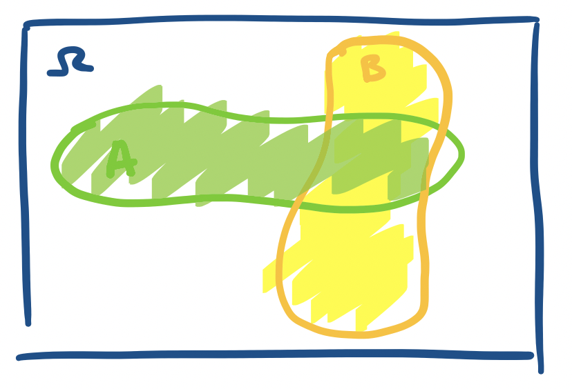
Because the sample space and events are just sets, we can often give "schematic" visual representations of them in the same way as sets. For example, the following is the sample space $\Omega$, which we treat in the same way as a universe, and events $A$ and $B$.
Intuitively, if we "throw a dart" at $\Omega$, then the probability that it lands in $A$ should be the $\Pr(A)$.
A sample space for flipping a coin would be whether it lands on heads and tails $\{H,T\}$. A sample space for the outcome of a die roll would be $\{1,2,3,4,5,6\}$. An event can be something simple like flipping a coin and it landing on heads, in which case the event would be the set $\{H\}$. It can also be more complicated, like a die roll landing on a square, which would be the set $\{1,4\}$, or perhaps the positive divisors of 6, which would be the set $\{1,2,3,6\}$.
For each sample space, we define a probability distribution, which tells us the probability of a particular event $\omega \in \Omega$. The simplest one is the uniform distribution.
The uniform distribution over a sample space $\Omega$ defines $\Pr(\omega) = \frac 1 {|\Omega|}$ for all $\omega \in \Omega$. Thus, $\Pr(A) = \frac{|A|}{|\Omega|}$.
Typically, this is the distribution we assume when we have an arbitrary finite set and say pick an element at random from our set—every item has an equal probability of being chosen:$\frac 1 n$ for $n$ elements, or $\frac{1}{|\Omega|}$.
In some sense, our picture of $\Omega$ and events $A$ and $B$ above is a bit inaccurate, because it depicts a continuous sample space. It might be better to make an explicitly discrete sample space. We can visualize this as a sample space that is broken up into discrete chunks.
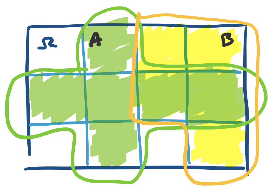
Here, we have the same idea, except we have discretized the space into 12 blocks, each of equal size. So now, we have $\Pr(A) = \frac 6{12} = \frac 1 2$ and $\Pr(B) = \frac{5}{12}$.
To determine the probability of an event (i.e. solve a problem), the textbook outlines a helpful process.
It's clear from above that the sample space for rolling one die is $\{1,2,3,4,5,6\}$, but what about two dice? Suppose we want to know the probability that our roll of two dice sums to 8.
What about coins? It turns out that flipping a bunch of coins is probably the most important sample space for theoretical comptuer science. Why? Let's try to do the same exercise as with dice. What if we want to represent a series of three coin flips? We can play the same game as with the dice: we have $\{H,T\} \times \{H,T\} \times \{H,T\}$ for our sample space. Now, if we were to generalize this to $n$ coin flips, we would have something like $\{H,T\}^n$. This space looks a lot more familiar if we rename $T = 0$ and $H = 1$, giving us the space $\{0,1\}^n$. That's right—the sample space of $n$ coin flips can be represented as the set of length $n$ binary strings!
Suppose we'd like to know for a series of 12 coin flips what the probability that we have exactly 8 heads is.
The view of a series of coin flips as binary strings is nice because it gives a bit of insight into how we might think of generating a random number. Typically, we think of a random number as something that we just "choose" "at random", but most people do not make choices that are truly uniformly at random. This suggests a better way of thinking about random numbers. First, figure out how large of a random number you want. Then flip a coin $n$ times, where $n$ is the size of your number. Then you have a binary string that you can interpret as a number!
This also suggests that creating a larger random number requires a "more" randomness and it gives us a way to think about randomness as a resource. If we need more coin flips, we are using more bits of randomness. We can then treat this quantity as a resource just like we do with time or space and ask how much randomness we might need for an algorithm and talk about the amount of randomness as a size of the input to the algorithm.
Recall that a standard deck of playing cards consists of four suits, $\spadesuit, \heartsuit, \clubsuit, \diamondsuit$ with cards numbered from 2 through 10, and a Jack, Queen, King, and Ace. This gives us 52 cards in total ($4 \times 13$). Suppose we want to know when drawing five cards what the probability that we can draw a flush is—that is, five cards of the same suit. (Technically a flush will exclude things like straight flushes, but we'll ignore that at this point)
Since we are dealing with sets, we can combine our sets in the same way as we've been doing to consider the probability of multiple events together. First, the following is a simple, but important bound.
$\Pr(A \cup B) \leq \Pr(A) + \Pr(B)$.
This follows directly from our understanding of sets. We have \begin{align*} \Pr(A \cup B) &= \frac{|A \cup B|}{|\Omega|} \\ &= \frac{|A| + |B| - |A \cap B|}{|\Omega|} \\ &= \frac{|A|}{|\Omega|} + \frac{|B|}{|\Omega|} - \frac{|A \cap B|}{|\Omega|} \\ &= \Pr(A) + \Pr(B) - \Pr(A \cap B) \\ &\leq \Pr(A) + \Pr(B) \end{align*}
Just like with sets, we can define the notion of disjointness for events.
Events $A$ and $B$ are disjoint if $A \cap B = \emptyset$.
$\Pr \left( \bigcup\limits_{i=1}^k A_i \right) \leq \sum_{i=1}^k \Pr(A_i)$. Furthermore, this is an equality if and only if the $A_i$ are pairwise disjoint.
This is just a generalization of the union bound and the proof comes straight from applying it. Alternatively, you can use induction to prove this. If you consider the events to be disjoint, this is really pretty much the sum rule. As you might have noticed, this result is due to George Boole, who is the same Boole that gave us Boolean algebra. Often times, this is also called the union bound.
There are a number of other useful properties that we can derive from set theory.
Let $A$ and $B$ be events. Then
Something that doesn't quite have a direct analogue from our discussions on set theory is the notion of conditional events. Arguably, this is what makes probability theory more than just fancy combinatorics.
If $A$ and $B$ are events, then the conditional probability of $A$ given $B$ is $$\Pr(A \mid B) = \frac{\Pr(A \cap B)}{\Pr(B)}.$$ Note that by this definition, $\Pr(A \cap B) = \Pr(A \mid B) \cdot \Pr(B)$.
One way of looking at this is if we restrict our attention to the event $B$, treat it like a sample space, and ask, what is the probability of $A$ in this space? In other words, what we're saying here is that if we know that $B$ already happened, then what is the probability that $A$ will happen? If we assume that our outcomes are uniformly distributed, then we can think about this in terms of sets: $$\Pr(A \mid B) = \frac{\Pr(A \cap B)}{\Pr(B)} = \frac{\frac{|A \cap B|}{|\Omega|}}{\frac{|B|}{|\Omega|}} = \frac{|A \cap B|}{|B|}.$$
If we look back at our diagram, we have the following.
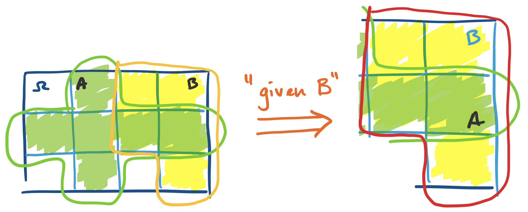
We can view this "globally" with respect to $\Omega$ and compute the probabilities: \[\Pr(A \mid B) = \frac{\Pr(A \cap B)}{\Pr(B)} = \frac{\frac{2}{12}}{\frac{5}{12}} = \frac 2 5.\] Or, if we jump straight into our observation above about "recentering" our space on $B$, we get that $\Pr(A \mid B) = \frac{|A \cap B|}{|B|} = \frac 2 5$ all the same.