There are a few ways we can rule out that graphs aren't the same, via properties that we call isomorphism invariants. There are properties of the graph that can't change via an isomorphism, like the number of vertices or edges in a graph.
One invariant that is not as obvious is the degree list of a graph. This is a list of all the degrees of the vertices. Clearly, if this list is different (say, one graph contains a vertex of degree 5 and the other doesn't), then the graphs are not isomorphic.
Sometimes we are not just interested in how some vertices may be related, but we are also interested in how vertices may be unrelated. Both are questions about the structure of the graph and lead to interesting properties.
A $k$-colouring of a graph is a function $c : V \to \{1,2,\dots,k\}$ such that if $(u,v) \in E$, then $c(u) \neq c(v)$. That is, adjacent vertices receive different colours. A graph is $k$-colourable if there exists a $k$-colouring for $G$.
Typically, we are concerned with the minimum number of colours required to colour a graph. An easy way to see why is to consider the following colouring for a graph of $n$ vertices: just colour each vertex its own colour.
The minimum number of colours for which a graph $G$ has a valid colouring is its chromatic number, denoted $\chi(G)$.
In other words, a graph $G$ is $k$-colourable if and only if $\chi(G) \leq k$.
We can use $k$-colourability as an invariant to show that two graphs are not isomorphic.
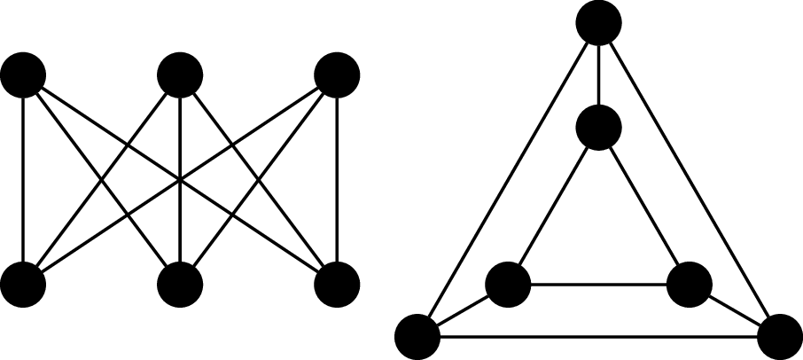
Consider the following two graphs, $G_1$ and $G_2$.
First, we observe that both graphs have 6 vertices and and 9 edges and both graphs are 3-regular. However, we will show that $G_1$ is 2-colourable and $G_2$ is not. To see that $G_1$ is 2-colourable, we observe that the vertices along the top row can be assigned the same colour because they are not adjacent to each other. Similarly, the vertices along the bottom can be assigned a second colour.
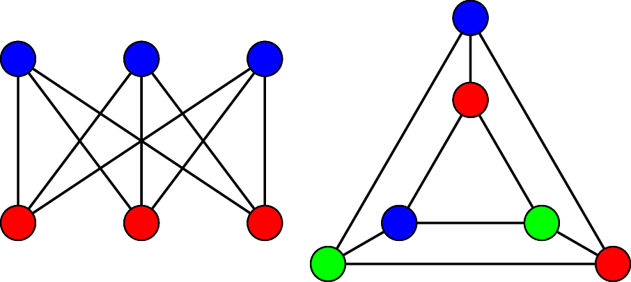
However, $G_2$ contains two triangles and by definition, the vertices belonging to the same triangle must be coloured with 3 different colours. Since $G_2$ is not 2-colourable, the adjacency relationship among the vertices is not preserved.
Historically, graph colouring was of interest in planar graphs. A graph is said to be planar if it can be drawn so that its edges don't intersect. Note that it's not enough to look at a drawing a graph to determine this—a planar graph can be drawn in a way that doesn't look planar, but could be drawn differently so it is. That said, there are graphs that are known not to be planar. One example is $K_5$, the complete graph on 5 vertices.
The main application for this was map colouring: how few colours do we need to colour a map so that two adjacent territories don't share the same colour? Such a map can be viewed as a planar graph, with vertices representing territories and edges representing whether the territories share a border.
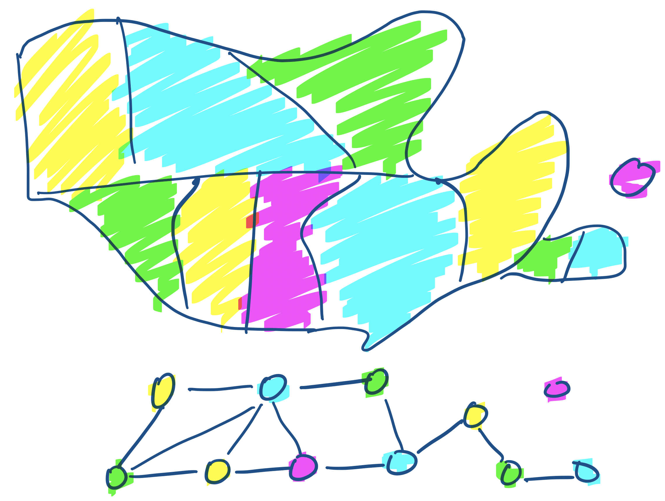
In this setting, the resulting graph is necessarily going to be planar. This is context for the most famous result in graph colouring: the Four Colour Theorem.
Every planar graph is 4-colourable.
This theorem was first conjectured in the mid-1800s but it wasn't until the 1970s that a proof, due to Appel and Haken, came about. The proof is of interest not just because it proved a long-standing open problem, but because it was the first case of the use of computers to assist in coming up with the proof.
To give you a sense of what's involved, here are some similar results and what their proofs are like.
The original proof by Appel and Haken had thousands of cases and the use of a computer to generate and verify those cases was controversial at the time. Part of this has to do with an underlying belief of many mathematicians that there must be a "nice" proof of such a nice statement. Unfortunately, we know there are true statements that have no proof and so it's not that far of a stretch to see that there must be true statements that have no "nice" or short proof—a consequence of what theoretical computer science tells us.
For the complete graph $K_n$, we have $\chi(K_n) = n$. Since every vertex in $K_n$ is adjacent to every other vertex, they're all forced to have their own colour.
Now, notice that the definition of the chromatic number talks about the minimum number of colours required. Does this mean that $K_n$ is, say, $n^2$-colourable? It turns out yes—recall that a $k$-colouring is a function $c : V \to \{1,\dots,k\}$. Notice there's no requirement for $c$ to be surjective—we don't have to use all the colours.
Thinking about this example of the complete graph, we can hypothesize that the maximum degree of a graph gives us an upper bound on the minimum colours we need to colour a graph.
Let $G$ be a graph with maximum degree $d$. Then $G$ is $(d+1)$-colourable.
Let $G = (V,E)$ be a graph with maximum degree $d$. We proceed by induction on $n = |V|$, the number of vertices in $G$.
Base case. We have $n = 1$. This is a graph with a single vertex, so the maximum degree of the graph is $0$. It is $1$-colourable, so our statement holds for the base case.
Inductive case. Let $k$ be an arbitrary positive integer and assume that for all graphs with $k$ vertices with maximum degree $d$, they are $(d+1)$-colourable. We let $G$ be a graph of $n = k+1$ vertices.
Choose an arbitrary vertex $v$ in $G$. We remove it and its incident edges to obtain a subgraph $H$ with $k$ vertices. All vertices in $H$ still have degree at most $d$, so $H$ is $(d+1)$-colourable by our inductive hypothesis. Let $c$ be our $(d+1)$-colouring for $H$.
Now, consider $G$. We construct a colouring $c'$ for $G$ by taking $c$ and assigning a colour to $v$. Since the maximum degree of vertices in $G$ is $d$, we have that $\deg(v) \leq d$. So we can choose from one of $d+1$ colours a colour for $v$ that is guaranteed to be different from its neighbours. This gives us a $(d+1)$-colouring $c'$ for $G$, so $G$ is $(d+1)$-colourable.
What does colouring tell us? Colouring is a way for us to partition the vertices of a graph. Vertices that receive the same colour are guaranteed not to be adjacent to each other—otherwise, they couldn't be the same colour.
A common application of this idea is in resource allocation problems, like scheduling. Suppose we are trying to schedule a bunch of exams. For instance, CMSC 27100, CMSC 25300, CMSC 14300, CMSC 14400, and CMSC 28100 are all courses that are offered this quarter. Four of those have combined exams, so scheduling them can be challenging and we need to check for conflicts.
We construct a graph assigning each course a vertex and drawing an edge between them if a student is taking both classes. In other words, each edge represents a conflict.
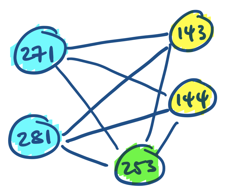
In this graph, we can guarantee that CMSC 27100 and CMSC 28100 are conflict free, since 271 is a prerequisite for 281. Similarly, no one can take 143 and 144 at the same time. In the end, we find that our graph is 3-colourable but not 2-colourable, so we need to reserve three different timeslots for these exams.
Here is another special type of graph. Recall that showing a graph is 2-colourable amounted to dividing the vertices up into two sets (or a partition) so that all of the edges of the graph only travel between these two sets. This gives us another special type of graph.
A graph $G = (V,E)$ is bipartite if $V$ is the disjoint union of two sets $V_1$ and $V_2$ such that all edges in $E$ connect a vertex in $V_1$ with a vertex in $V_2$. We say that $(V_1, V_2)$ is a bipartition of $V$.
We get the following characterization of bipartite graphs for free from the definition of 2-colourability.
A graph $G$ is bipartite if it is 2-colourable.
Suppose $G = (V,E)$ is bipartite, with bipartition $(V_1, V_2)$. Then we can define a 2-colouring $c:V \to \{1,2\}$ by $c(v) = i$ iff $v \in V_i$, for $i = 1,2$. In other words, assign all the vertices in $V_1$ one colour and assign all the vertices in $V_2$ the other colour. Since there are no edges between any vertices in the same side of the partition, we know that we can assign them all the same colour.
Now, suppose $G = (V,E)$ is 2-colourable. So there is a colouring $c:V \to \{1,2\}$. Then we define the bipartition $(V_1, V_2)$, where $V_1 = \{v \in V \mid c(v) = 1\}$ and $V_2 = \{v \in V \mid c(v) = 2\}$. That is, we take the vertices of one colour as one side of the bipartition and the vertices of the other colour to be the other side. Since edges can only be incident to vertices of different colours and there are only two colours, we have that $(V_1, V_2)$ is a bipartition.
Similar to the idea of complete graphs, we can define complete bipartite graphs.
The complete bipartite graph on $m$ and $n$ vertices is the graph $K_{m,n} = (V,E)$, where $(V_m,V_n)$ is a bipartition of $V$ with $|V_m| = m$ and $|V_n| = n$, and $$E = \{(u,v) \mid u \in V_m, v \in V_n \}.$$
The bipartite graph from Example 18.4 above is the complete bipartite graph $K_{3,3}$. This graph also happens to be the other usual example of a graph that isn't planar.