Graph Theory
You may be familiar with graphs as either graphical charts of data or from calculus in the form of visualizing functions in some 2D or 3D space. Neither of these are the graphs that are discussed in graph theory.
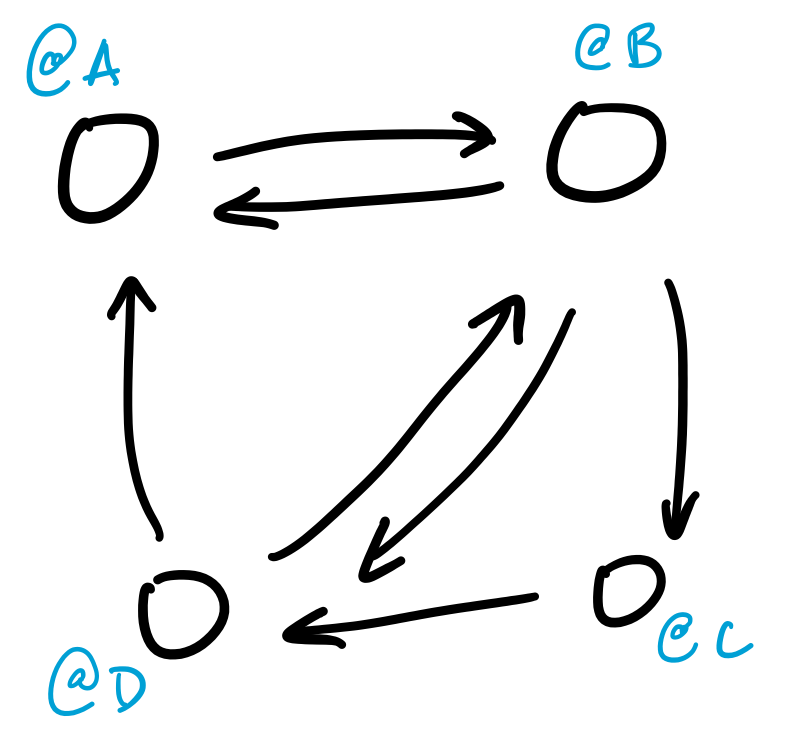
Graphs have a natural visual representation: we represent things as circles, which we call nodes or vertices, and we represent a relationship between two things by drawing a line or arrow between them, which we call edges.
Perhaps some of the most obvious graphs in our lives nowadays are those related to the Internet:
A social network is a graph, where the vertices are people or accounts and the edges are some kind of relationship (friends, followers, etc.). When given this structure, we might want to locate large friend groups and influencers, by looking for cliques, or computing nodes with high centrality.
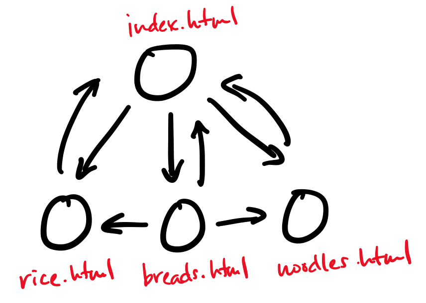
The web is a graph, where the vertices are webpages and the edges are links from one page to another. This model of the web is what informs many web search algorithms, like Google's PageRank, which measures the importance of a webpage based on how many incoming and outgoing links it has.
The Internet itself is a graph, where the vertices are the physical computers and the edges are the physical connections between them. Many computer networks can be viewed in this way. A common question that one can ask from this perspective is about minimum cuts. This is the question of what the cheapest way to disconnect the graph is, and therefore sever the network. This is a measure of the robustness of a network.
Graphs also have lots of non-network applications in computer science.
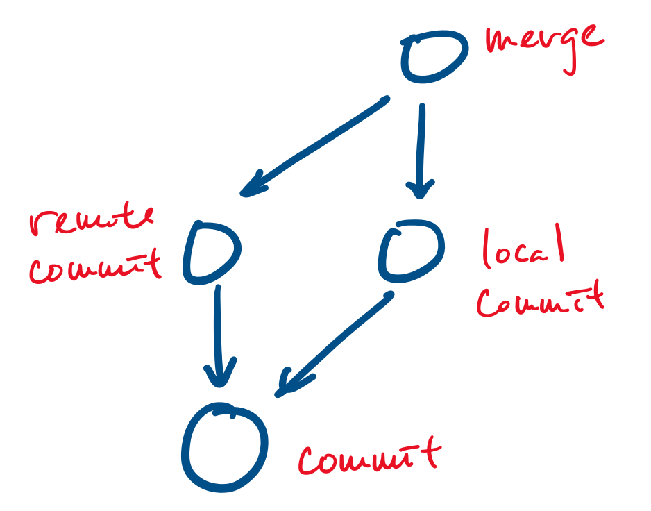
Your favourite revision control system, git, uses a graph based data model: all objects (such as files and commits) are represented as vertices and edges point from an object to an object that they depend on. For example, a commit is represented as a vertex and a merge can be represented as a vertex that points to the commits it merges.
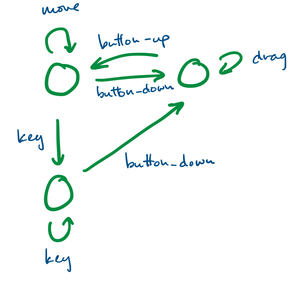
Finite state systems are often represented as graphs. These model the behaviour of complex systems, like software. For example, we can imagine that a program is in a "wait" state until a certain button has been pressed, at which point it moves to the appropriate state.
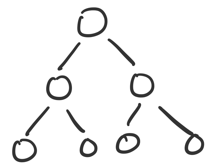
We've already made heavy use of a specific kind of graph: the binary tree. Trees, in general, are a class of graphs, specifically those that do not contain any cycles.
Graphs also model many real-world phenomena.
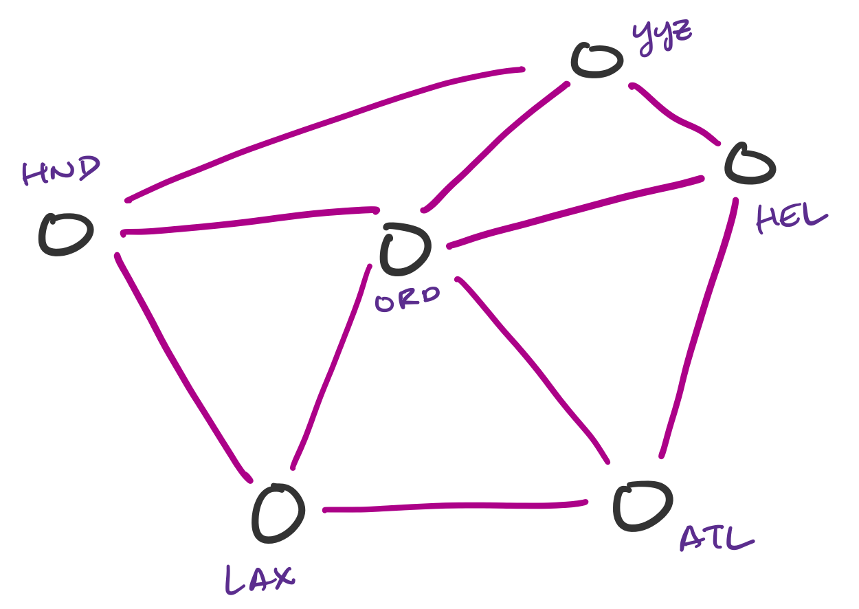
Transportation networks are commonly represented as graphs. These are not necessarily physical traffic networks, but more conceptual ones, like a flight network or a public transit network. One can then ask questions about the lowest-cost path from one node in the network to another.
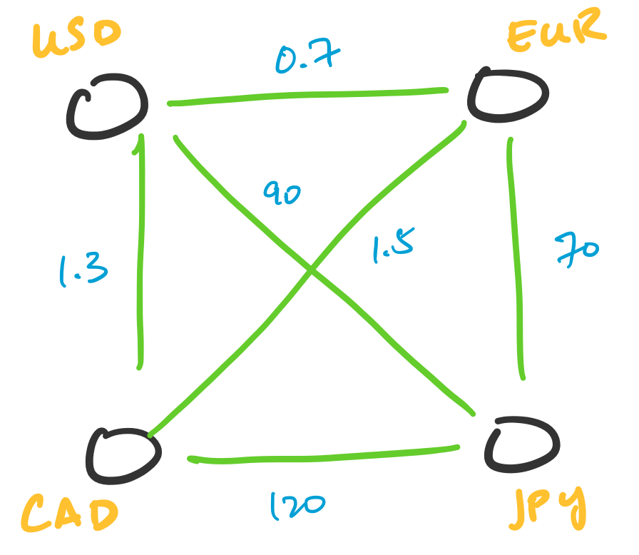
Transactions can be represented as graphs. One particularly interesting application of this is in currency arbitrage. In this setting, we represent currencies as vertices and assign weights to the edges corresponding to the exchange rate between two currencies. What makes this interesting is the fact that exchange rates can be totally independent of each other, which leads to opportunities for arbitrage. This involves indentifying cycles of a particular weight.
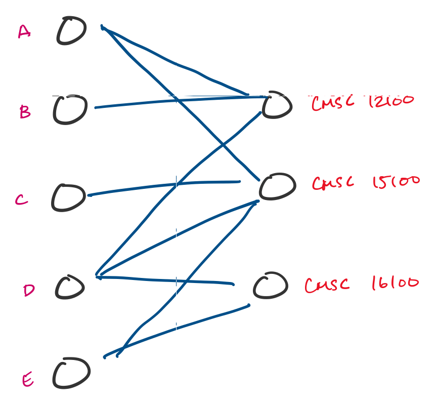
Many tasks can be reformulated as graphs. For instance, resource allocation is something that doesn't look like a graph problem, but can be turned into one. Suppose a university is trying to enroll students into classes in an upcoming quarter and students submit preferences for classes they would like to take. This can be modeled using a graph, and a possible assignment is a choice of a subset of edges.
You'll be familiar with the concept of graphs if you've taken courses in the introductory CS sequence. There, you are introduced to graphs as a data structure. Here, we'll be considering graphs as a mathematical object. As we've been seeing, this is actually not so different, except that we don't really have any "implementation details" to think about.
A graph $G = (V,E)$ is a pair with a non-empty set of vertices $V$ together with a set of edges $E$. An edge $e \in E$ is an unordered pair $(u,v)$ of vertices $u,v \in V$.
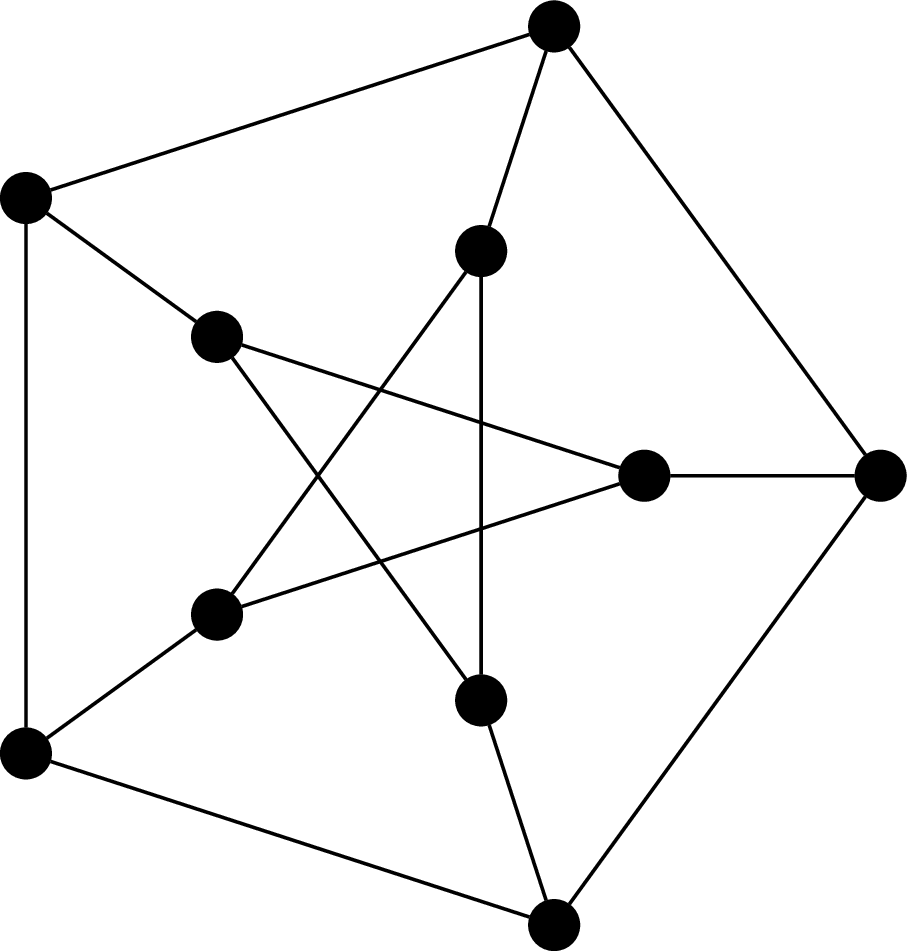
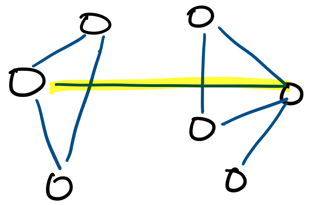
This graph is called the Petersen graph. The Petersen graph is a particularly interesting graph, not just because it looks neat, but because it happens to be a common counterexample for many results in graph theory.
From the definition, we immediately get that the edge set $E$ is a relation on $V \times V$. Furthermore, for undirected graphs, the edge relationship is always symmetric: $(u,v) \in E \rightarrow (v,u) \in E$. However, we don't treat these two pairs as different edges—they are considered one and the same.
One can define graphs more generally and then restrict consideration to our particular definition of graphs, which would usually be then called simple graphs. Instead, what we do is start with the most basic version of a graph, from which we can augment our definition with the more fancy features if necessary (it will not be necessary in this course).
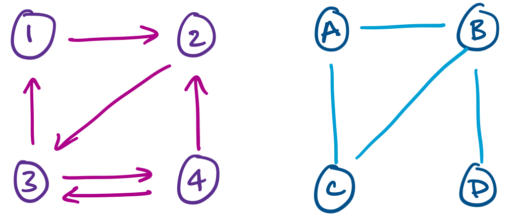
For example, the above examples indicate that we can have a version of graphs in which edges have a direction, or where the edge relation is not enforced to be symmetric. These are directed graphs.
More general definitions of graphs also allow for things like multiple edges between vertices or loops.
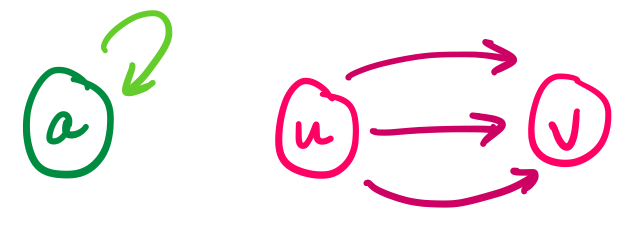
Other enhancements may include equipping edges with weights or even generalizing edges to hyperedges that relate more than two vertices.
Two vertices $u$ and $v$ of a graph $G$ are adjacent if they are joined by an edge $(u,v)$. We say the edge $(u,v)$ is incident to $u$ and $v$. The degree of a vertex $v$ in $G$, denoted $\deg(v)$, is the number of its neighbours.
In other words, adjacency is about the relationship between two vertices, while incidence is about the relationship between a vertex and an edge.
The following results are some of the first graph theory results, proved by Leonhard Euler in 1736.
Let $G = (V,E)$ be an undirected graph. Then
$$\sum_{v \in V} \deg(v) = 2 \cdot |E|.$$
Every edge $(u,v)$ is incident to exactly two vertices: $u$ and $v$. Therefore, each edge contributes 2 to the sum of the degrees of the vertices in the graph.
Now, let's look at some examples of some well-known graphs.
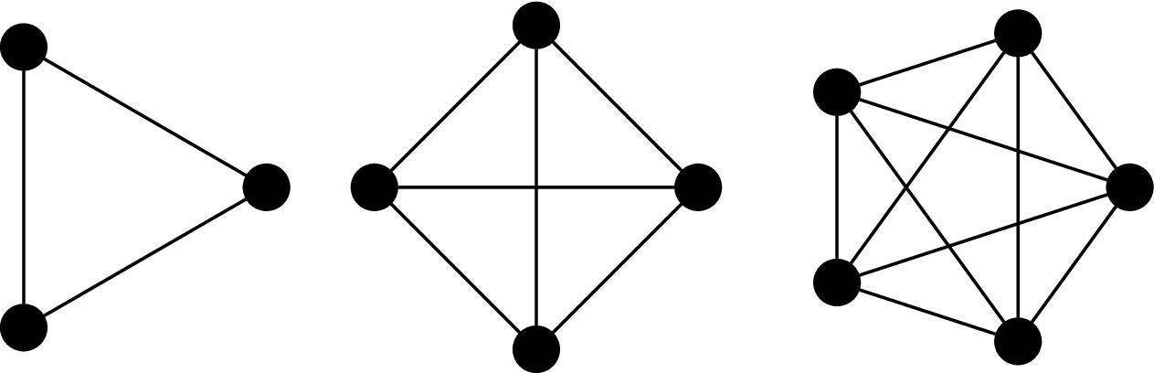
The complete graph on $n$ vertices is the graph $K_n = (V,E)$, where $|V| = n$ and
$$E = \{(u,v) \mid u,v \in V\}.$$
That is, every pair of vertices are neighbours.
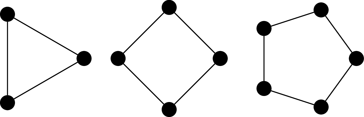
The cycle graph on $n$ vertices is the graph $C_n = (V,E)$ where $V = \{v_1, v_2, \dots, v_n\}$ and $E = \{(v_i,v_j) \mid j = i + 1 \bmod n\}$. It's named so because the most obvious way to draw the graph is with the vertices arranged in order, on a circle.
The $n$-(hyper)cube graph is the graph $Q_n = (V,E)$, where $V = \{0,1\}^n$ (i.e., binary strings of length $n$) and $(u,v)$ is an edge if, for $u = a_1 a_2 \cdots a_n$ and $v = b_1 b_2 \cdots b_n$, there exists an index $i, 1 \leq i \leq n$ such that $a_i \neq b_i$ and $a_j = b_j$ for all $j \neq i$. In other words, $u$ and $v$ differ in exactly one symbol.
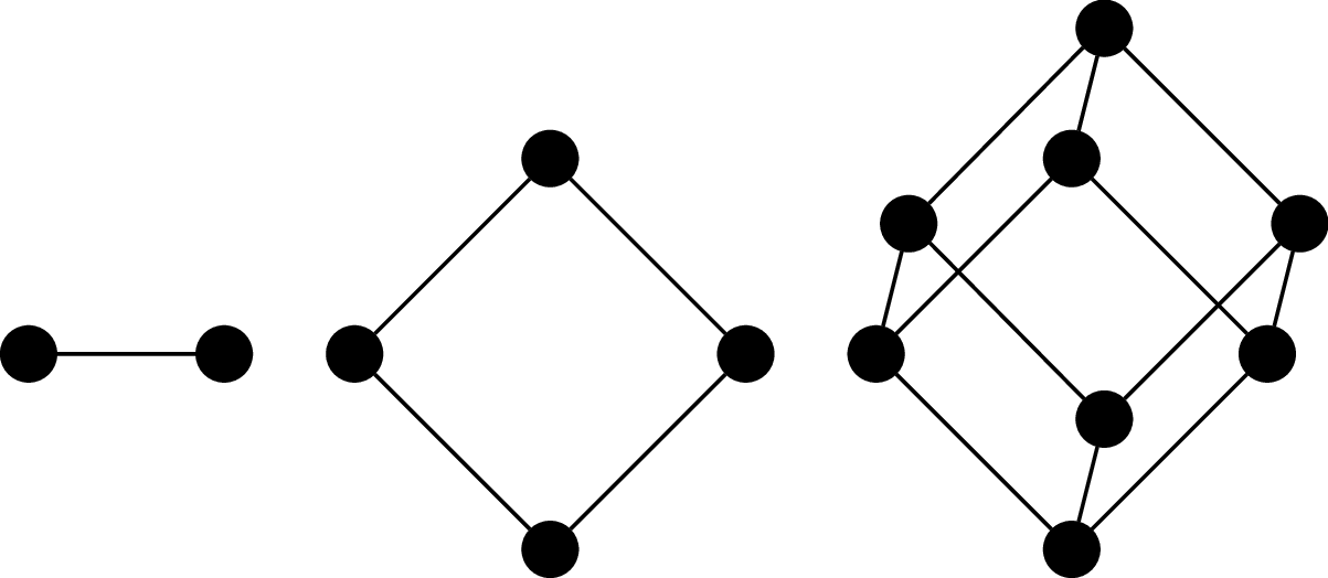
It's called a cube (or hypercube) because one of the ways to draw it is to arrange the vertices and edges so that they form the $n$th-dimensional cube.
Graph isomorphism
Consider the following graphs.
These two graphs happen to be the "same". Furthermore, it turns out that these are also basically the same graph as $Q_3$, or at least, we feel that it should be. This means we don't need to necessarily draw a $3$-cube like a cube (and we certainly wouldn't expect this for $n \gt 3$).
Although the visual representation of the graph is very convenient, it is sometimes misleading, because we're limited to 2D drawings. In fact, there is a vast area of research devoted to graph drawing and the mathematics of embedding graphs in two dimensions. The point of this is that two graphs may look very different, but turn out to be the same.
But even more fundamental than that, we intuitively understand that just because the graph isn't exactly the same (i.e., the vertices are named something differently) doesn't mean that we don't want to consider them equivalent. So how do we discuss whether two graphs are basically the same, just with different names or drawings?
An isomorphism between two graphs $G_1 = (V_1,E_1)$ and $G_2 = (V_2,E_2)$ is a bijection $f:V_1 \to V_2$ which preserves adjacency. That is, for all vertices $u,v \in V_1$, $(u,v) \in E_1$ if and only if $(f(u),f(v) \in E_2$. Two graphs $G_1$ and $G_2$ are isomorphic if there exists an isomorphism between them, denoted $G_1 \cong G_2$.
In other words, we consider two graphs to be the "same" or equivalent if we can map every vertex to the other graph such that the adjacency relationship is preserved. In practice, this amounts to a "renaming" of the vertices, which is what we typically mean when we say that two objects are isomorphic. Of course, this really means that the edges are preserved.
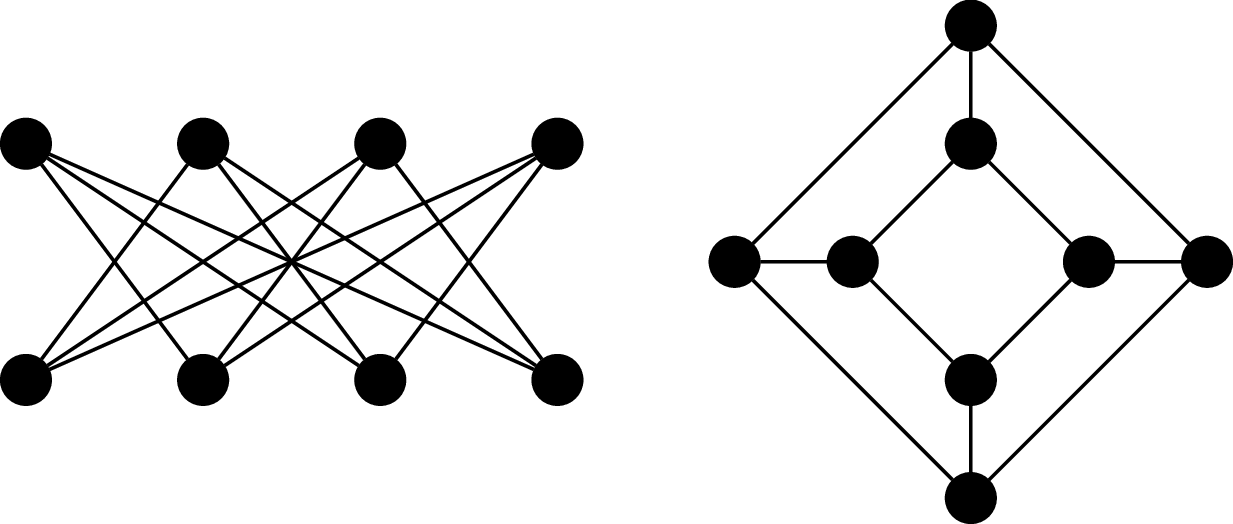
Consider the following graphs $G_1 = (V_1, E_1)$ and $G_2 = (V_2, E_2)$.
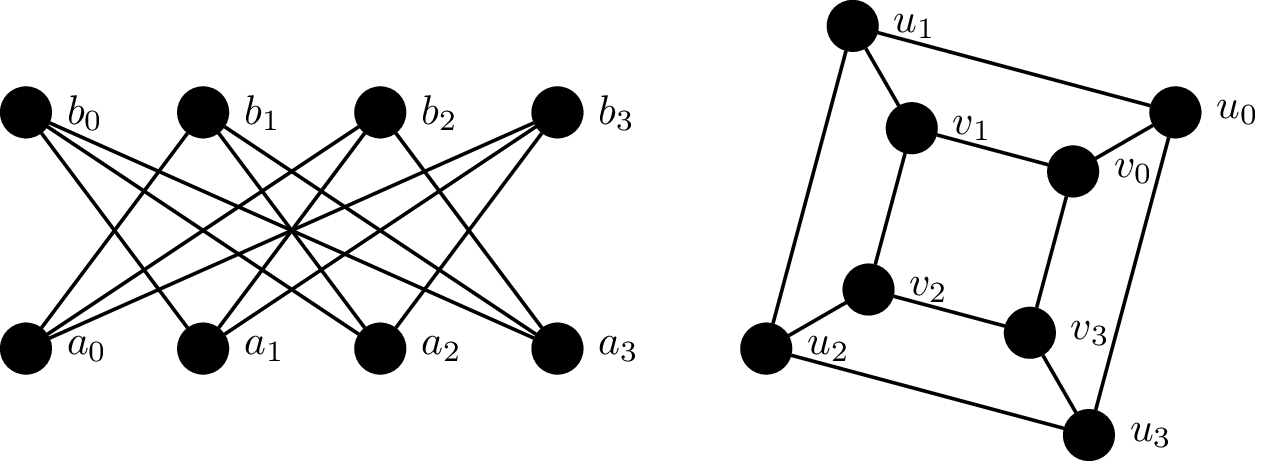
We will show that these two graphs are isomorphic by defining a bijective function $f:V_1 \to V_2$ which preserves adjacency:
\begin{align*}
f(a_0) &= u_0 & f(a_1) &= v_3 & f(a_2) &= u_2 & f(a_3) &= v_1 \\
f(b_0) &= v_2 & f(b_1) &= u_1 & f(b_2) &= v_0 & f(b_3) &= u_3 \\
\end{align*}
This is a bijection, since every vertex in $V_1$ is paired with a vertex in $V_2$. We then verify that this bijection preserves adjacency by checking each edge under the bijection:
\begin{align*}
(f(a_0),f(b_1)) &= (u_0,u_1) & (f(a_0),f(b_2)) &= (u_0,v_0) & (f(a_0),f(b_3)) &= (u_0,u_3) \\
(f(a_1),f(b_0)) &= (v_3,v_2) & (f(a_1),f(b_2)) &= (v_3,v_0) & (f(a_1),f(b_3)) &= (v_3,u_3) \\
(f(a_2),f(b_0)) &= (u_2,v_2) & (f(a_2),f(b_1)) &= (u_2,u_1) & (f(a_2),f(b_3)) &= (u_2,u_3) \\
(f(a_3),f(b_0)) &= (v_1,v_2) & (f(a_3),f(b_1)) &= (v_1,u_1) & (f(a_3),f(b_2)) &= (v_1,v_0)
\end{align*}
So an obvious and fundamental problem that arises from this definition is: Given two graphs $G_1$ and $G_2$, are they isomorphic? The obvious answer is that we just need to come up with an isomorphism or show that one doesn't exist. Unfortunately, there are $n!$ possible such mappings we would need to check.